Computational Graphs and Automatic Differentiation

Understanding the mathematical foundations of Deep Learning is crucial to mastering neural networks and optimization techniques. At the core of this field lie computational graphs and automatic differentiation, which enable efficient gradient computation and optimization in modern machine learning models.

This article introduces the concept of computational graphs and explores the automatic differentiation techniques used to compute gradients, including forward mode differentiation and reverse mode differentiation (backpropagation). These methods are essential in training neural networks and are widely implemented in frameworks such as PyTorch.

This article is part of the Deep Learning Foundations series, which covers fundamental topics essential for understanding deep learning. If you are looking for a structured introduction to deep learning concepts, check out Deep Learning Foundations.

Now, let’s dive into computational graphs, differentiation techniques, and their role in training neural networks.

Consider a function $f$ that depends on some parameters $\theta$ : $f(x | \theta)$ . We have a set of input-output pairs, $(x_0, y_0), (x_1, y_1), \ldots, (x_n, y_n)$ . For each input-output pair, we can define an error function $E$ that measures the difference between the output of $f$ and the actual value $y$ . Specifically, the error function can be expressed as:

$L(y, \bar{y}) = L(y_0, f(x_0 | \theta))$

Our goal is to find the value of $\theta$ that minimizes the error $L$ on average:

$\min_{(x_i, y_i) \in D} \mathbb{E}[L(y_i, f(x_i | \theta))]$

One effective way to find the optimal parameters $\theta$ is by using the Stochastic Gradient Descent (SGD) method.

Gradient Computation

To minimize the error, we need to compute the gradient of the error with respect to the parameters, $\frac{\partial L}{\partial \theta}$ . The expected value of this gradient, $\mathbb{E}\left[ \frac{\partial L}{\partial \theta} \right]$ , has the same dimensionality as $\theta$ and points in the direction that maximizes $L$ . To minimize $L$ , we take steps in the opposite direction of the gradient:

$\theta_{t+1} = \theta_t - \eta \cdot \mathbb{E}\left[ \frac{\partial L}{\partial \theta} \right]$

where $\eta$ is the learning rate, which controls the step size.

Methods to Compute Gradients

There are several ways to compute the gradient $\frac{\partial L}{\partial \theta}$ :

Manual Differentiation: This involves computing gradients by hand. While feasible for simple functions, it becomes impractical for complex or deep networks.
Symbolic Differentiation: This method uses symbolic algebra systems to compute exact derivatives. However, it can be computationally expensive or even impossible for very large models.
Automatic Differentiation (Autograd): This is the preferred method in machine learning. It combines numerical efficiency with the ability to handle complex models.

A Simple Machine Learning Model

A simple machine learning model can be represented as a sequence of layers:

$\text{Input} \rightarrow \text{Layer 1} \rightarrow \text{Layer 2} \rightarrow \text{Layer 3} \rightarrow \text{Output}$

This can be formalized as:

$y = f_3(f_2(f_1(x)))$

This operation is called function composition and can also be written as $f_3 \circ f_2 \circ f_1$ .

Chain Rule and Backpropagation

For a composition of functions, the derivative can be computed using the chain rule. For example, consider:

$h(x) = f(g(x))$

The derivative $h'(x)$ is given by:

$h'(x) = f'(g(x)) \cdot g'(x)$

Unfolding the equation for $y = f_3(f_2(f_1(x)))$ :

$\begin{aligned}z_1 &= f_1(x) \\z_2 &= f_2(z_1) \\y &= f_3(z_2)\end{aligned}$

The derivative of $y$ with respect to $x$ is then:

$\frac{\partial y}{\partial x} = \frac{\partial y}{\partial z_2} \cdot \frac{\partial z_2}{\partial z_1} \cdot \frac{\partial z_1}{\partial x}$

This process, which involves multiplying the partial derivatives, is fundamental to backpropagation in neural networks.

Binary Operators

A binary operator is a rule for combining two elements (called operands) to produce another element

$f: A \times B \rightarrow C$

A binary operator is closed if its domain is $A \times A$ and its codomain is $A$ . The closed operator in $\mathbb{R}$ are:

Addition
Multiplication
Subtraction
Division

Every binary operator cause a split in the derivation flow. In $\mathbb{R}$ every closed binary operator create a summation of two derivation flows:

$\frac{\partial (f(x) + g(x))}{\partial x} = \frac{\partial f(x)}{\partial x} \text{\color{red}{+}} \frac{\partial g(x)}{\partial x}$

$\frac{\partial (f(x) \cdot g(x))}{\partial x} = g(x) \cdot \frac{\partial f(x)}{\partial x} \text{\color{red}{+}} f(x) \cdot \frac{\partial g(x)}{\partial x}$

$\frac{\partial (f(x) - g(x))}{\partial x} = \frac{\partial f(x)}{\partial x} \text{\color{red}{+}} - \frac{\partial g(x)}{\partial x}$

$\frac{\partial (\frac{f(x)}{g(x)})}{\partial x} = \frac{1}{g(x)} \cdot \frac{\partial f(x)}{\partial x} \text{\color{red}{+}} - \frac{f(x)}{g(x)^2} \cdot \frac{\partial g(x)}{\partial x}$

Computational Graphs

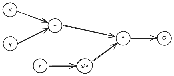
Computational graphs are a powerful tool for visualizing and performing differentiation on complex functions. Each node in the computational graph represents an operation, and the edges represent the flow of data between these operations.

Binary Operator Differentiation

Binary operators such as addition, subtraction, multiplication, and division play a crucial role in computational graphs. When differentiating a computational graph that contains binary operators, each operator creates a split in the differentiation flow. Consider the following function:

$(x + y) \cdot \sin(z)$

To represent this as a computational graph:

Computational Graph (x+y)sin(z)

For binary operators, we treat the differentiation as follows:

Addition (+): The derivative of the output with respect to each input is simply $1$ . For example, the partial derivative $\frac{\partial (x + y)}{\partial x} = 1$ and $\frac{\partial (x + y)}{\partial y} = 1$ . This means that when backpropagating, the gradient is distributed equally across both inputs.
Subtraction (-): The derivative with respect to the first operand is $1$ , and with respect to the second operand is $-1$ . For example, $\frac{\partial (x - y)}{\partial x} = 1$ and $\frac{\partial (x - y)}{\partial y} = -1$ . During backpropagation, the gradient flows positively to the minuend and negatively to the subtrahend.
Multiplication ( $\times$ ): The derivative depends on both inputs. The partial derivative with respect to is the value of $y$ , and vice versa. For example, $\frac{\partial (x \cdot y)}{\partial x} = y$ and $\frac{\partial (x \cdot y)}{\partial y} = x$ . This means that during backpropagation, each input receives the gradient multiplied by the value of the other input.
Division ( $\div$ ): The derivative with respect to the numerator is $1/y$ , and with respect to the denominator is $-x/y^2$ . For example, $\frac{\partial (x / y)}{\partial x} = \frac{1}{y}$ and $\frac{\partial (x / y)}{\partial y} = -\frac{x}{y^2}$ . During backpropagation, the gradient is scaled by the reciprocal of the denominator for the numerator, and scaled negatively for the denominator.

Each binary operator in the computational graph results in a split in the flow of derivatives, which must be summed accordingly when propagating back through the graph. Note that, if there are some coefficients, such as $2x$ , the representation in the computational graph can be simplified by considering the coefficient as a separate node in the graph.

Forward Differentiation

In forward mode differentiation, the derivatives are propagated from inputs to outputs, following the flow of the computational graph. This method is particularly useful when the number of inputs is smaller than the number of outputs, as it allows efficient computation of all partial
derivatives with respect to a single input.
Consider the same example:

$(x + y) \cdot \sin(z)$

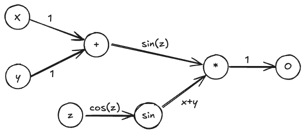
Let’s proceed by building the computational graph, writing down the partial derivatives at each step (on each edge, it is written the derivative of the successive node with respect to the previous node):

Computational Graph (x+y)sin(z) with derivatives

Here is how the differentiation proceeds step by step:

At the addition node (+), we propagate the partial derivative of $y$ with respect to $x$ and $y$ , which are both $1$ . The output of the addition node has a derivative of $1$ with respect to each of its inputs.
At the sine node ( $\sin(z)$ ), the derivative with respect to $z$ is computed as $\cos(z)$ . This value is then used in the next step to propagate through the multiplication node.
At the multiplication node ( $\times$ ), we apply the chain rule. The partial derivative with respect to the output of the addition node is $\sin(z)$ , and the derivative with respect to the output of the sine node is $(x + y)$ . The derivative value is propagated through the edges to the final output node.

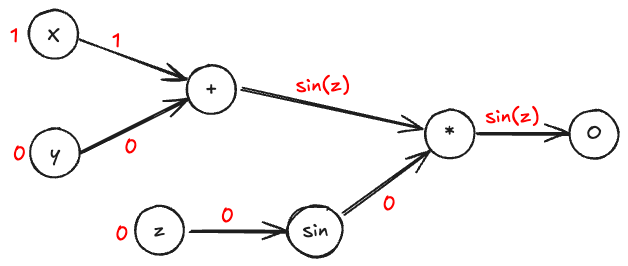
The forward mode differentiation allows us to compute the derivative of the output with respect to each input parameter in a single pass through the computational graph. Given the partial derivatives at each step, we can efficiently compute the gradient of the output with respect to all input parameters. In the following, the computational graph is represented to show the flow of derivatives from an input to the output. The derivatives are computed at each step and propagated forward through the graph.

Computational Graph (x+y)sin(z) forward

We obtain that the derivative of the output with respect to $x$ is $sin(z)$ .

Reverse Differentiation

Reverse mode differentiation, also known as backpropagation, is more efficient when dealing with functions where the number of inputs is much larger than the number of outputs. In machine learning, this is often the case as models may have thousands or millions of parameters (inputs) but produce a single scalar loss (output).
Consider the same function:

$(x + y) \cdot \sin(z)$

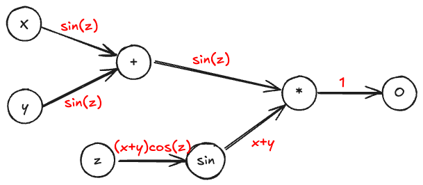
In reverse mode differentiation, we begin by computing the derivative of the final output with respect to itself, which is $1$ . We then propagate this derivative backward through each node in the graph:

At the multiplication node ( $\times$ ), we distribute the gradient to each of its inputs. The derivative with respect to $(x + y)$ is $\sin(z)$ , and the derivative with respect to $\sin(z)$ is $(x + y)$ .
At the sine node ( $\sin(z)$ ), we propagate the gradient back by multiplying it with the derivative of $\sin(z)$ , which is $\cos(z)$ .
At the addition node (+), the gradient is equally split between $x$ and $y$ since $\frac{\partial (x + y)}{\partial x} = 1$ and $\frac{\partial (x + y)}{\partial y} = 1$ .

The process continues until all input nodes have received their respective gradient contributions. This allows us to efficiently compute the gradient of the output with respect to every input parameter in a single backward pass. The computational graph for reverse differentiation can be represented as follows:

Computational Graph (x+y)sin(z) backward

If we want to compute the derivative of the output with respect to $x$ , we can follow the reverse differentiation process:

$\frac{\partial y}{\partial x} = 1 \cdot \sin(z) \cdot 1 = \sin(z)$

Or, if we want to compute the derivative of the output with respect to $z$ :

$\frac{\partial y}{\partial z} = 1 \cdot (x + y) \cdot \cos(z) = (x + y) \cos(z)$

This representation clearly shows how the gradients flow backward through the computational graph, allowing efficient computation of all required derivatives.

Numerical Differentiation Frameworks

There are several numerical differentiation frameworks available that utilize reverse mode differentiation under the hood. These frameworks provide high-level APIs to easily construct complex machine learning models. Popular frameworks include:

These frameworks allow users to define computational graphs and automatically compute gradients, making it easier to implement and train deep learning models.

import torch
import math

x = torch.tensor([math.pi], requires_grad=True)
y = torch.tensor([math.pi], requires_grad=True) 

o = (x + y) * torch.sin(x) 
o.backward() 

print(x.grad) # Output: tensor([-6.2832]) 
print(y.grad) # Output: tensor([-8.7423e-08])

Code Is Broken

Computational Graphs and Automatic Differentiation

Gradient Computation

Methods to Compute Gradients

A Simple Machine Learning Model

Chain Rule and Backpropagation

Binary Operators

Computational Graphs

Binary Operator Differentiation

Forward Differentiation

Reverse Differentiation

Numerical Differentiation Frameworks

Lascia un commento Annulla risposta